A Tutorial on Clustering Algorithms

Introduction | K-means | Fuzzy C-means | Hierarchical | Mixture of Gaussians | Links

Clustering as a Mixture of Gaussians

Introduction to Model-Based Clustering
There’s another way to deal with clustering problems: a model-based approach, which consists in using certain models for clusters and attempting to optimize the fit between the data and the model.
In practice, each cluster can be mathematically represented by a parametric distribution, like a Gaussian (continuous) or a Poisson (discrete). The entire data set is therefore modelled by a mixture of these distributions. An individual distribution used to model a specific cluster is often referred to as a component distribution.

A mixture model with high likelihood tends to have the following traits:

• component distributions have high “peaks” (data in one cluster are tight);
• the mixture model “covers” the data well (dominant patterns in the data are captured by component distributions).

Main advantages of model-based clustering:

• well-studied statistical inference techniques available;
• flexibility in choosing the component distribution;
• obtain a density estimation for each cluster;
• a “soft” classification is available.

Mixture of Gaussians
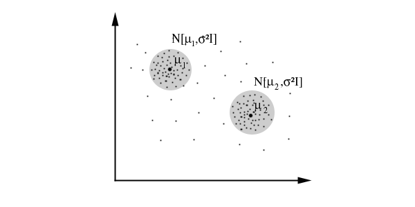
The most widely used clustering method of this kind is the one based on learning a mixture of Gaussians: we can actually consider clusters as Gaussian distributions centred on their barycentres, as we can see in this picture, where the grey circle represents the first variance of the distribution:

The algorithm works in this way:

• it chooses the component (the Gaussian) at random with probability ;
• it samples a point .

Let’s suppose to have:

• x₁, x₂,..., x_N
• 

We can obtain the likelihood of the sample: .
What we really want to maximise is (probability of a datum given the centres of the Gaussians).

is the base to write the likelihood function:

Now we should maximise the likelihood function by calculating , but it would be too difficult. That’s why we use a simplified algorithm called EM (Expectation-Maximization).

The EM Algorithm
The algorithm which is used in practice to find the mixture of Gaussians that can model the data set is called EM (Expectation-Maximization) (Dempster, Laird and Rubin, 1977). Let’s see how it works with an example.

Suppose x_k are the marks got by the students of a class, with these probabilities:

x₁ = 30            

x₂ = 18            

x₃ = 0              

x₄ = 23            

First case: we observe that the marks are so distributed among students:

x₁ : a students
x₂ : b students
x₃ : c students
x₄ : d students

We should maximise this function by calculating . Let’s instead calculate the logarithm of the function and maximise it:

Supposing a = 14, b = 6, c = 9 and d = 10 we can calculate that .

Second case: we observe that marks are so distributed among students:

x₁ + x₂ : h students
x₃ : c students
x₄ : d students

We have so obtained a circularity which is divided into two steps:

• expectation:
• maximization:

This circularity can be solved in an iterative way.

Let’s now see how the EM algorithm works for a mixture of Gaussians (parameters estimated at the pth iteration are marked by a superscript (p):

Bibliography

Previous page | Next page